Species interactions
In the previous tutorials we studied a single species interacting with a fixed background community. In this tutorial we want to acknowledge that there is no such thing as a fixed background community. Instead, all species form part of a dynamical ecosystem in which changes to any species has knock-on effects on other species. Furthermore, the resulting changes in the other species will react back on the first species, which now finds its prey community and its predator community changed. This is where we realise that we need multi-species models, because without such a model we cannot predict how all these changes will affect each other.
Trait-based model
In this first part of the course we aim for understanding, not realism. So in this tutorial we investigate the tangled web of interactions in an idealised multi-species system. We choose a trait-based model in which the species making up the community differ from each other only in a single trait: their asymptotic body size (sometimes it is also called maximum body size).
We use the newTraitParams() function to create our idealised trait-based multi-species model. The function has many parameters, but we will just keep the defaults. Unlike the newSingleSpeciesParams() function, the newTraitParams() function does not set the initial spectra to their steady state values. We thus need to run the result through the steady() function. We assign the resulting MizerParams object to the variable mp.
mp <- newTraitParams() |> steady()Let us look at the biomass density in log weight.
plotSpectra(mp, power = 2, total = TRUE)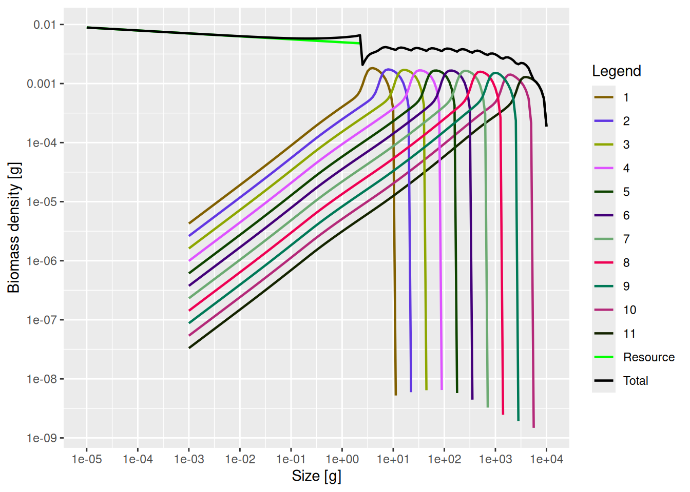
We see 11 species spectra and a resource spectrum. The resource spectrum starts at a smaller size than the fish spectra, in order to provide food also for the smallest individuals (larvae) of the fish spectra. Each species spectrum has a shape of the type we expect, given what we have seen in the tutorial on single species spectra. The spectra of the different species all look essentially the same, except for being shifted along the size axis. This is because in this trait-based model the species differ only through their asymptotic size. This regularity will of course not be present in a real-world ecosystem, but it makes it easier for us to build an intuition about the effects of species interactions.
Note how the community size spectrum, plotted in black, that is obtained by summing together all the individual species and resource spectra, approximately follows a power law (i.e., approximately follows a straight line in the log-log plot).
Turn off reproduction dynamics
As in previous tutorials, we want to concentrate on the shapes of the size spectra and we do not yet want to look at what determines the overall abundance of each species. Therefore we modify the model so that it keeps the abundances at egg size fixed (i.e. numbers in the first size bin). You do not need to look in detail at the following code, except to note that a mizer model is very customisable in the sense that an advanced user can overwrite almost any behaviour with custom behaviour.
mp <- mp |>
    setRateFunction("RDI", "constantEggRDI") |>
    setRateFunction("RDD", "noRDD")
The functionality for customising and extending mizer will be the subject of an entire extra part of this course. But in the meantime you can certainly let us know what kinds of customisation you would like to make in the comments section and we can give pointers. You can also look at a recent blog post where Phoebe Woodworth-Jefcoats shows how to use custom rate functions to implement temperature-dependent rates in mizer.
Mortality from other species
The species interact with each other via predator-prey interactions. These interactions shape both mortality and energy income. In this section we look at mortality imposed on a particular species by its predators. We choose to look at species 8. The following graph shows the relative contributions to the mortality rate for species 8 from all the other species:
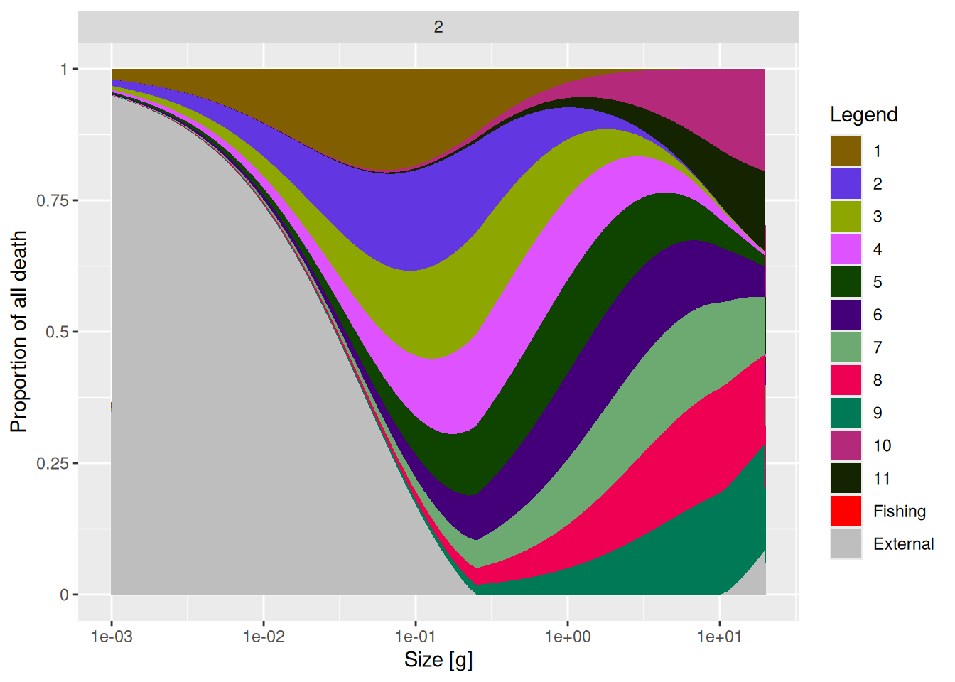
plotlyDeath(mp, species = "8")The horizontal axis shows the size of the individual whose mortality we are looking at. Towards the left we see the mortality of the small larvae, as we move towards the right we move to larger individuals. So the main important message from this graph is that as an individual grows up their main predators change.
You might have expected that species 8 would be predated upon by the larger species 9, 10 and 11. And for large individuals of species 8, these three species do indeed form the dominant source of predation mortality, but we see also that smaller individuals of species 8 are predominantly predated upon by predators from smaller species. This arises because each predator prefers to feed at a certain fraction of its own size (which is set to 1/100th in this model), so the larger predators loose interest in the larvae and concentrate on the larger prey.
This ontogenetic diet shift as an individual grows up is one reason why standard food-web models, where interaction between predator and prey is entirely determined by their species, are insufficient for modelling fish communities.
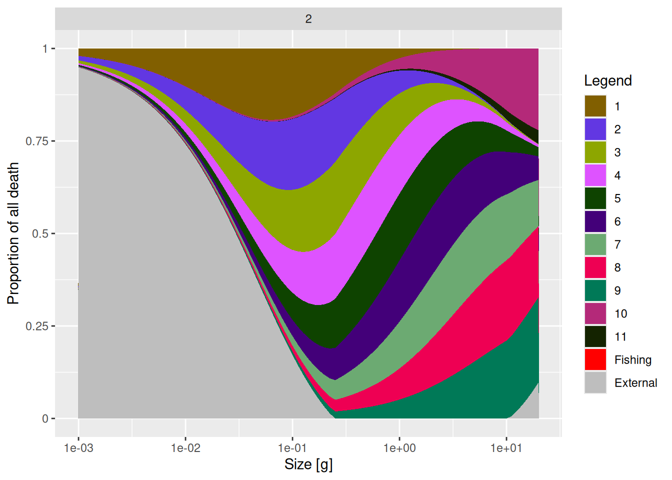
In the above graph you also see that the smallest individuals and the largest individuals get the majority of their mortality from “external” sources, by which we designate all the mortality that is not from predation by the modelled species. So it is “external” in the sense that its sources are not represented inside the model. For large individuals this external mortality would include predation from mammals and seabirds as well as senescence mortality. For small individuals this external mortality comes from predation by small, possibly planktonic, organisms that are not explicitly modelled.
In the absence of other information, our simple trait-based model just assumes that this external mortality is such that the total mortality scales allometrically with an individual’s size to the power of -1/4. This is why larval mortality is actually quite high. We can see this in the following plot which instead of proportions shows the actual mortality rates:
plotDeath(mp, species = "8", proportion = FALSE)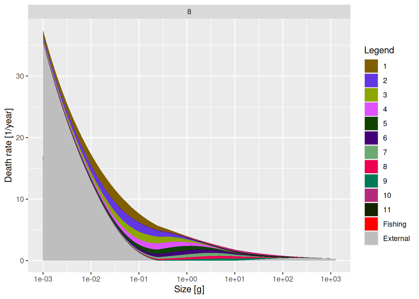
The plotDeath() function is extremely useful when building your own model. It is important to know where the majority of mortality on your species and its various sizes come from.
Income from other species
Now that we have investigated who eats species 8, we also want to know who is eaten by species 8. We can check that by plotting the diet of this species:
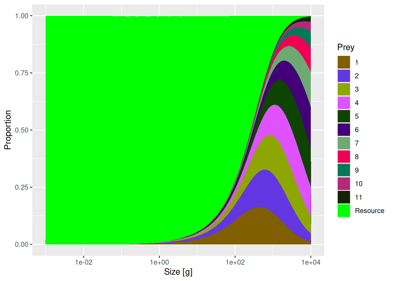
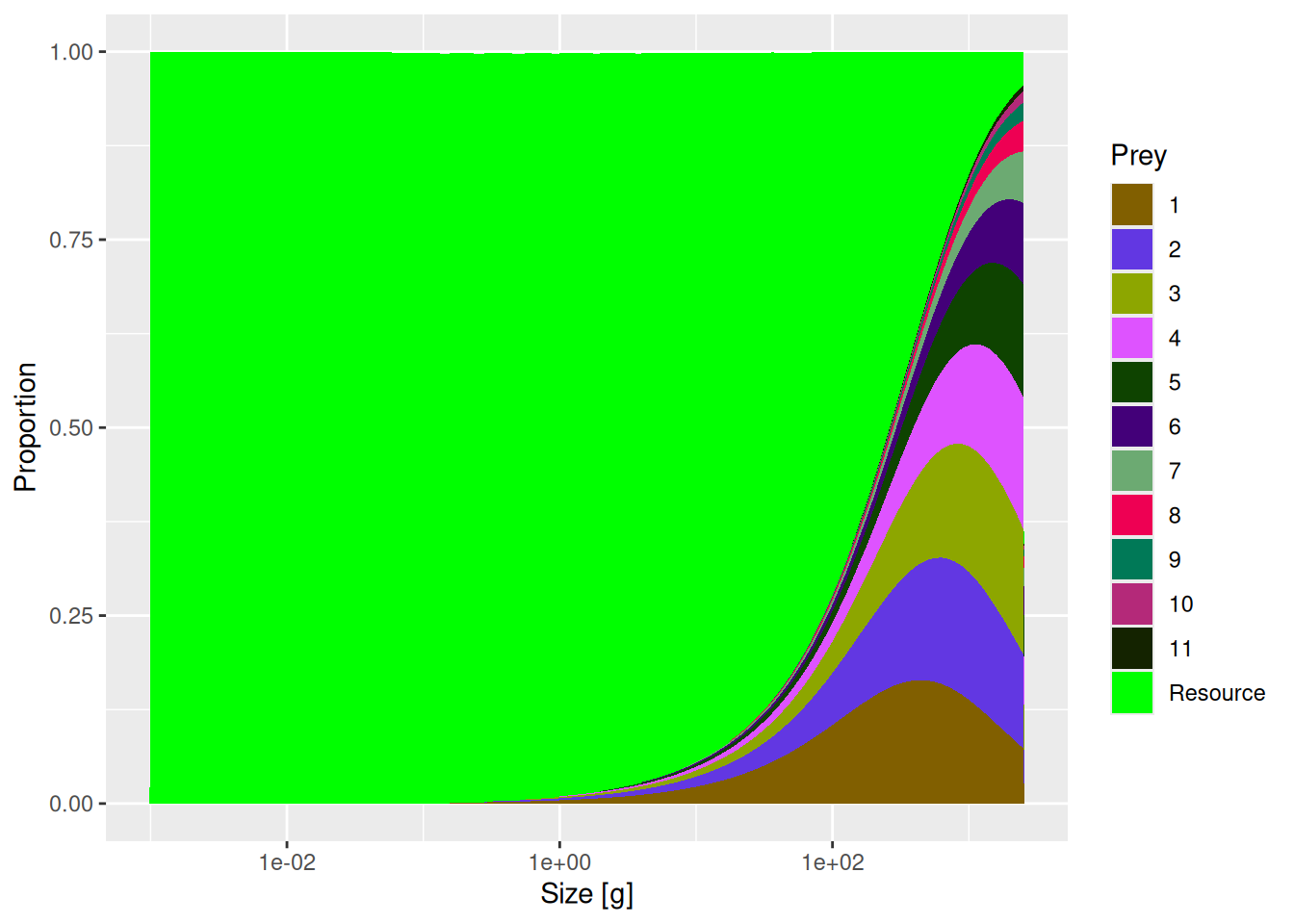
plotDiet(mp, species = "8")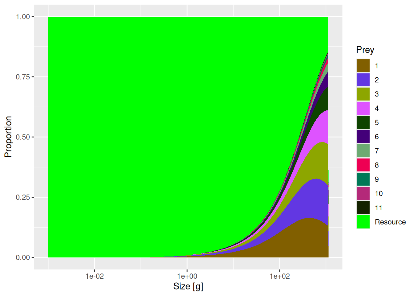
The diet looks quite reasonable. Small individuals of species 8 initially feed entirely on the resource (plankton and other small things). From about the size of 1g (which is roughly 4-5 cm) they start eating also larvae of other fish.
The diet composition we see in the plot is shaped by two things: the predation kernel (the size preference in the feeding of the predator) and the relative abundances of prey at different sizes. First, a predator will only eat food that is within the predation kernel size range. But once in this size range the relative proportion of different species or resource consumed will simply depend on their relative biomass. So if, for example, 80% of biomass in a specific prey size class consists of resource, 15% of species 1 and 5% of species 2, then the diet of the predator feeding in that size class will consist of 80% resource, 15% of species 1 and 5% of species 2.
In our example model, resource abundance at small size classes is very high compared to abundance of fish. So when a predator feeds in those size classes, naturally most of the diet will consist of resource. This is what we see in the diet plot.
Of course, when we build a model for a real-world ecosystem we will have some knowledge about the biology of the species and their food preferences. Perhaps one species is actively selecting fish out of the resource, or predating on specific species only? This is where the interaction matrix comes in that we will discuss in the next section.
It is very important to explore diets of species in your model, so, like the plotDeath() function, the plotDiet() function is very useful.
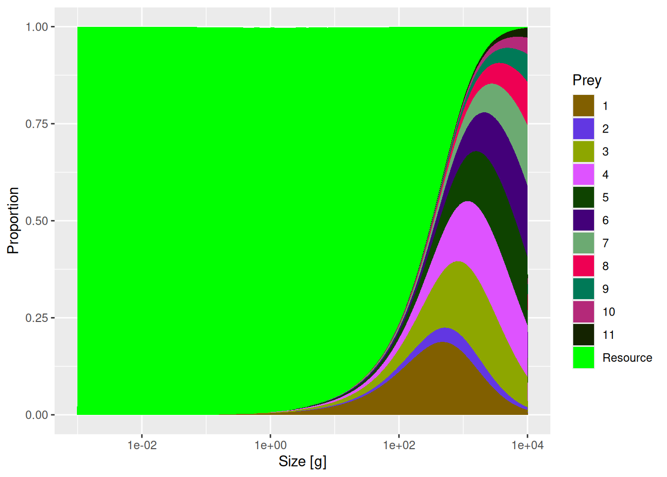
Now, check what the diets of other species look like by making a plot for each species from 1 (smallest one) to 11 (the largest one). Hint: if you look at the documentation for plotDiet() you may find a convenient way to do this.
plotDiet(mp)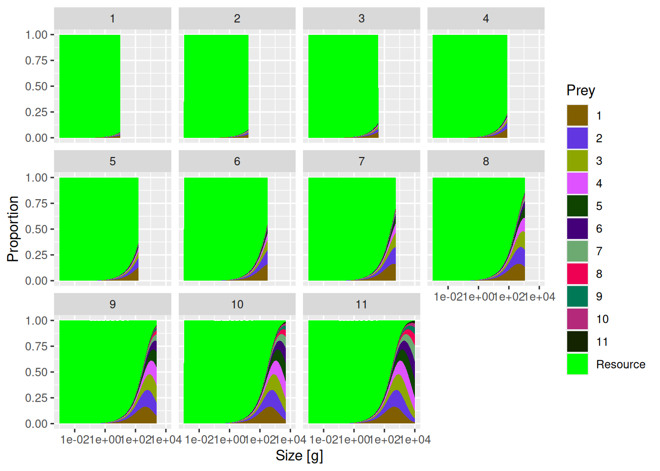
Interaction matrix
Now we arrive to an interesting and challenging aspects of multi-species modelling - setting up parameters for species and resource interactions. By default, mizer assumes that all species in the model can access all other species and resource equally and the amount of different prey consumed just depends on their relative abundance in the predator’s feeding size range. So the default interaction matrix of the species in our model looks very simple
        prey
predator 1 2 3 4 5 6 7 8 9 10 11
      1  1 1 1 1 1 1 1 1 1  1  1
      2  1 1 1 1 1 1 1 1 1  1  1
      3  1 1 1 1 1 1 1 1 1  1  1
      4  1 1 1 1 1 1 1 1 1  1  1
      5  1 1 1 1 1 1 1 1 1  1  1
      6  1 1 1 1 1 1 1 1 1  1  1
      7  1 1 1 1 1 1 1 1 1  1  1
      8  1 1 1 1 1 1 1 1 1  1  1
      9  1 1 1 1 1 1 1 1 1  1  1
      10 1 1 1 1 1 1 1 1 1  1  1
      11 1 1 1 1 1 1 1 1 1  1  1
The matrix has all values set at 1 which means that all predators can access all prey species equally.
In reality we might have some knowledge about predators’ diet preferences, or about prey vulnerability to predation. This knowledge should be incorporated in the interaction matrix. Perhaps we know that some predators cannot or do not eat certain prey. For example some species in our system might only feed on plankton and never ever eat any fish. In this case we will set all values in the row for that predator equal to 0. Or we might know that some prey is less available to predation due to some anti-predation behaviour or defence mechanisms. In this case we would decrease all values in the prey column to something < 1.
You should not set an entry in the interaction matrix to 0 just because a particular prey is never recorded in the stomach of a predator. It may well be that the predator species consumes the larvae of the prey species at some stage of their life and these larvae are simply not recorded in the stomach content.
The interaction matrix can encode lots of effects. Sometimes the interaction matrix is used to encode spatial overlap of species in a large ecosystem, as in this application of mizer to the North Sea. In this case the interaction matrix might be estimated from spatial surveys assessing species spatial overlap.
Let’s go ahead and change one value in the interaction matrix.
mp_modified <- mp
# We change row 11 (predator species 11) and column 2 (prey species 2)
# to a smaller value
interaction_matrix(mp_modified)[11, 2] <- 0.2
Now let’s compare the source of mortality for species 2 in the two models.
You will see a reduction of the contribution of species 11 to the mortality of species 2.
Next let us compare diets of species 11 in the two models.
You will see a reduction in the contribution of species 2 to the diet of species 11. By setting the entry in row 11 and column 2 of the interaction matrix to 0.2 we simply reduced the availability of prey species 2 for predator species 11 by a factor of 5. The entries in the interaction matrix simply serve as multipliers on the available prey biomass.
Resource interactions
The interaction coefficients between the fish species as consumers and the resource as food, which one could have expected to find in an additional column in the interaction matrix, is instead saved as a species parameter.
species_params(mp)$interaction_resource 1 2 3 4 5 6 7 8 9 10 11
1 1 1 1 1 1 1 1 1 1 1 We see that the default value for all these interaction coefficients is also 1.
Now we might want to reduce the availability of resource to some predators. Perhaps we know that certain species much prefer to feed on other fish rather than on similar sized plankton. Let us look at an example where species 8 through 11 have a 20% reduction in their interaction with resource.
# We make a copy of the model
mp_lessRes <- mp
# and set the resource interaction to 0.8 for species 8 to 11
given_species_params(mp_lessRes)$interaction_resource[8:11] <- 0.8
# We print out the result to check
species_params(mp_lessRes)$interaction_resource
1 2 3 4 5 6 7 8 9 10 11
1.0 1.0 1.0 1.0 1.0 1.0 1.0 0.8 0.8 0.8 0.8 Now we can look at the diet of for example species 9 and compare it with the previous model
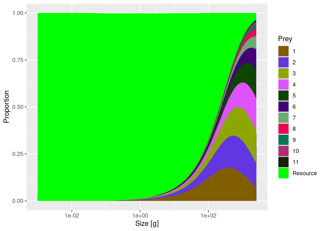
The change seems small enough. However, now that we changed the availability of resources, which is so important for larval stages, these four species will experience a much reduced growth rate during their juvenile stage. We can see that effect by recalculating the single-species spectra with
mp_lessRes_sss <- steadySingleSpecies(mp_lessRes)and then ploting the spectra
plotSpectra(mp_lessRes_sss, power = 2)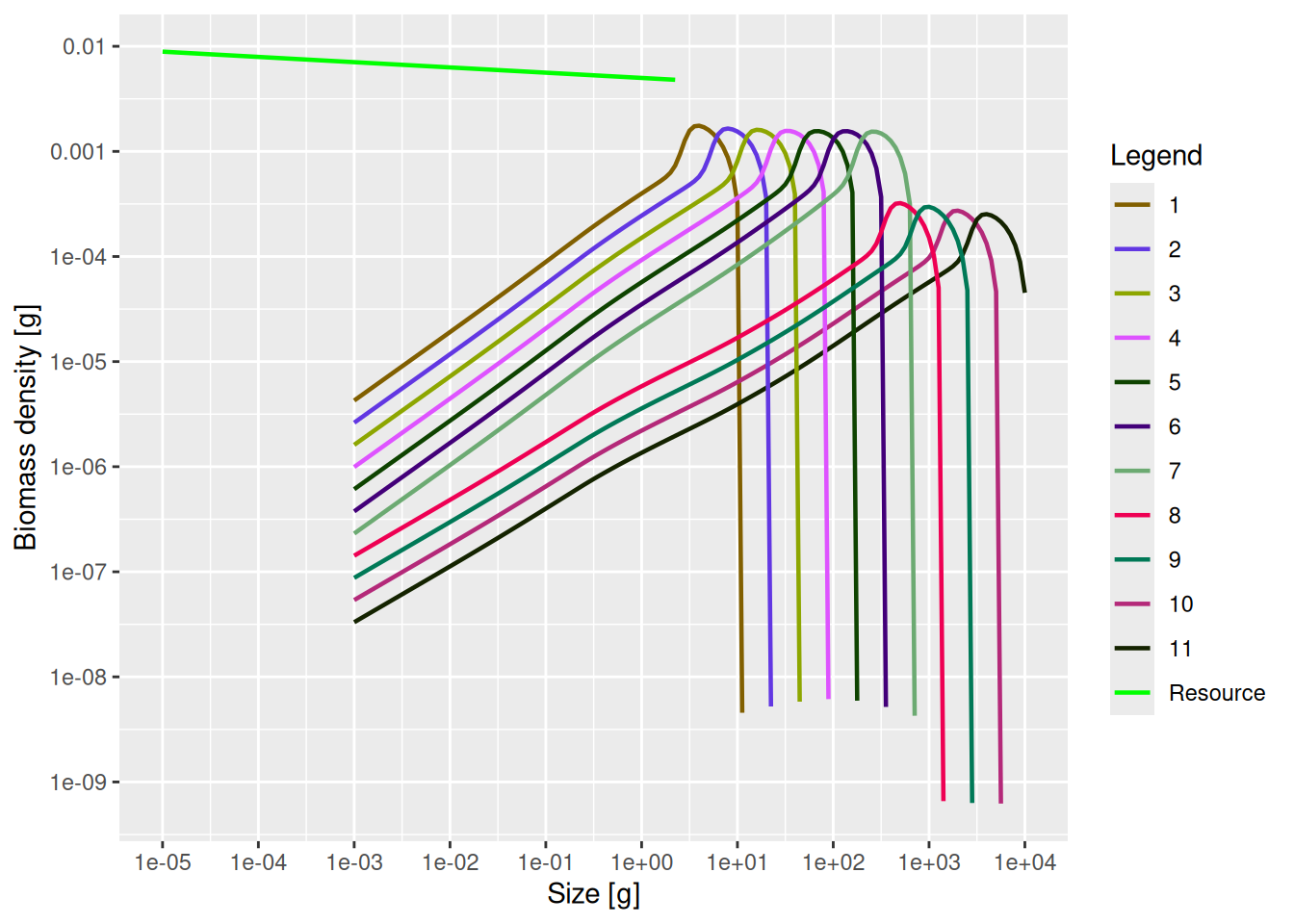
We can see the drastic reduction in the abundances of species 8 to 11.
It is very important to understand that the above picture does not represent what will actually happen in the multi-species model. The above picture represents single-species thinking. We changed something for species 8 to 11 and then calculated the effect that change has on those species assuming they stayed in the same environment with the same prey and predator abundances. But of course the rest of the ecosystem will react, as we will now investigate.
Trophic cascades
As we just discussed, the above picture does does not show a steady state of the ecosystem. Species now find themselves with a different abundance of predators and prey and this will change their mortality and their growth and hence their size spectra.
The easiest way to find the new steady state that the ecosystem will settle into is to simulate the full multi-species dynamics forward in time. Mizer refers to this simulation to find the future state of the ecosystem as “projecting”. We can use the function projectToSteady() to project forward in time far enough so the system has settled down again close to the new steady state.
mp_lessRes_steady <- projectToSteady(mp_lessRes)Convergence was achieved in 24 years.plotSpectra2(mp_lessRes_steady, name1 = "less resource",
mp, name2 = "original",
total = TRUE, power = 2, ylim = c(1e-8, NA), wlim = c(1e-3, NA))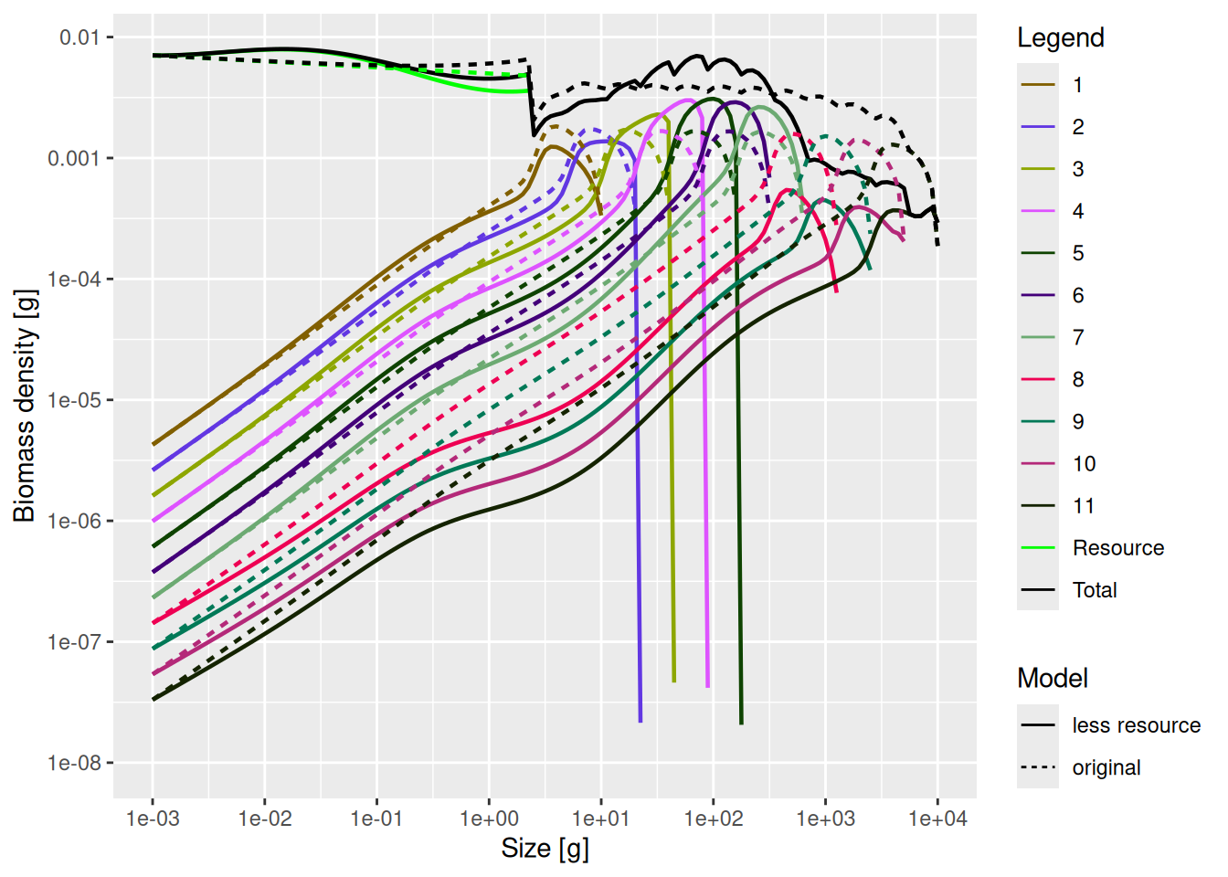
There is much to see in this graph. We can see how the reduction in the abundance of large individuals leads to undulations in fish and resource size spectra, compared to the original model.
Fishing-induced cascades
Let’s investigate these trophic cascades a bit more. This time we can look at how fishing large fish will affect the ecosystem.
The model has been set up with a knife-edge fishing gear that selects all individuals above 1kg, irrespective of species. This is not a realistic gear and mizer can do much better, as we will see in Part 3. But it serves our current purpose, because it will impose a fishing mortality that only impacts the larger species that actually grow to sizes above 1kg. To use that gear we just have to set a non-zero fishing effort. We create a new model mp_fishing with a fishing effort of 1:
mp_fishing <- mp
initial_effort(mp_fishing) <- 1
As we did in the section on fishing mortality in the previous tutorial, we can visualise the direct effect that this fishing mortality has on individual species:
mp_fishing_sss <- steadySingleSpecies(mp_fishing)
plotSpectra(mp_fishing_sss, power = 2)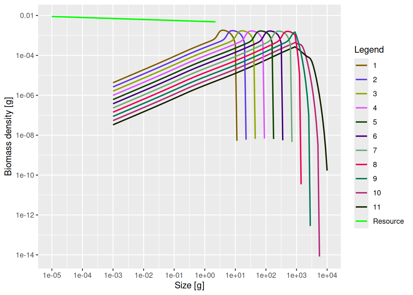
As expected, the largest species have their abundances reduced above 1kg if they are fished, and if they continue to encounter the same amount of prey and are exposed to the same amount of predation mortality.
Again the important point is that the above picture does does not show a steady state of the ecosystem. You will look at the multi-species steady state in the next exercise to see if this fishing also leads to a trophic cascade.
Project the mp_fishing model to its steady state and then make a plot comparing it to the steady state of the un-fished system. Do you see a trophic cascade?
mp_fishing_steady <- projectToSteady(mp_fishing_sss)Convergence was achieved in 12 years.plotSpectra2(mp, name1 = "No fishing",
mp_fishing_steady, name2 = "Fishing",
power = 2,
wlim = c(1e-2, NA), ylim = c(1e-6, NA))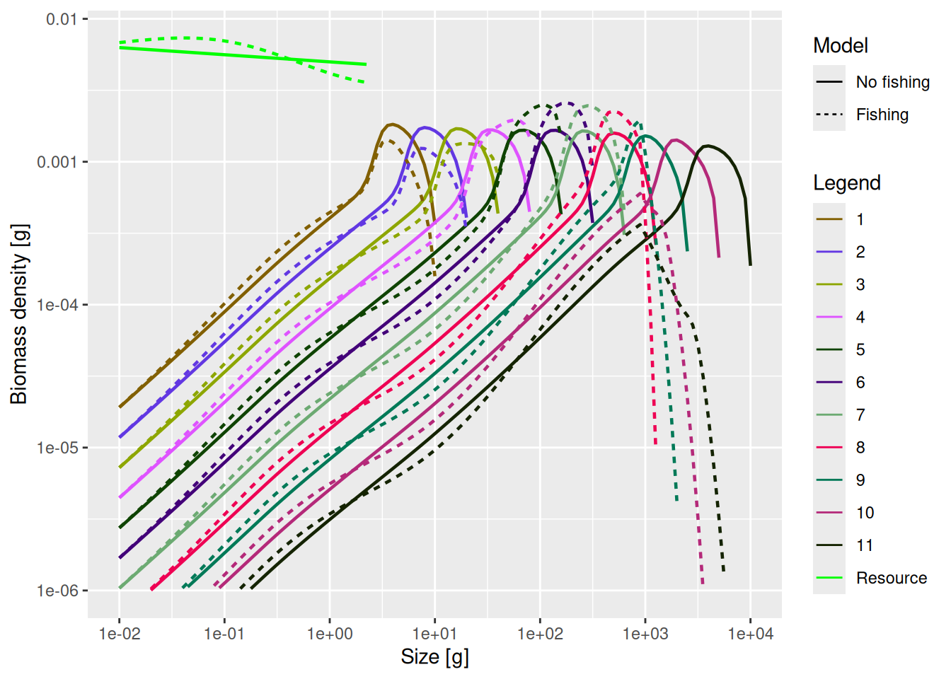
There is a clear trophic cascade.
Summary and recap
When using mizer models it is very important to investigate who eats whom and where mortality comes from. We do this with the functions
plotDeath()andplotDiet().The contribution of different species to the diet of a predator depends on the abundances of the species in the size range preferred by the predator.
The species interaction matrix defines availability of each species to predation by other species. By changing the interaction matrix we can make our models more realistic and more complex.
Trophic cascades are one of the coolest things in multi-species models and the reason we build these models. We want to understand how changes in one species and its sizes will affect the whole ecosystem. Mizer has many ways how we can explore such trophic cascades.